In order to measure the effects of an intervention, the immediate, step, and ramp effects are measured using statistical linear models. Using linear models to measure the effects in an interrupted time-series are useful for a few reasons.
Interpretability: The coefficients (β) have straightforward interpretations like baseline level, trend, and the magnitudes of different intervention effects.
Underlying Trend: Often, pre-intervention time series exhibit a roughly linear trend, making the linear model suitable.
Flexibility: Even with some non-linearity, the segmented structure of the model (pieces before and after the interruption) can still give a good approximation of change.
6.2 Linear Equation
The following equation is a common way to represent interrupted time series analysis in a statistical model.
T: Time, progressing incrementally throughout your study period.
D: A dummy variable, ‘0’ before the intervention, ‘1’ after, representing the intervention itself.
P: Time since the intervention, starting at 0 before the intervention.
β_0: The baseline trend of your outcome before the intervention and time.
β_1: The ‘pre-intervention slope’ of the outcome before the intervention.
β_2: The immediate change in the outcome level right at the point of intervention.
β_3: The difference in the trend (slope) between the pre-intervention and post-intervention periods (e.g., the difference in the slope after the intervention compared to the expected slope had the intervention not happened).
ϵ: Random error unaccounted for by the model.
6.3 Statistical Models
The choice of method can affect the level and slope change point estimates, their standard errors, width of confidence intervals, and p-values. Some possible choices include ordinary least squares (OLS), Newey-West (NW), Prais-Winsten (PW), restricted maximum likelihood (REML), and autoregressive integrated moving average (ARIMA) models.
6.3.1 Ordinary Least Squares (OLS)
The classic linear regression model. It finds the line that best fits the data by minimizing the squared differences between observed values and predicted values. While usable for some ITS analysis, OLS is often problematic because time series data frequently violates the assumption of independent errors. Autocorrelation, if present, leads to underestimated standard errors and potentially misleading conclusions. OLS for ITS assumes residuals are independent (no autocorrelation) with constant variance.
6.3.2 Newey-West (NW)
Also a linear regression method, but specifically designed to address autocorrelation. It adjusts the standard errors of the model coefficients to be robust to autocorrelation (and some heteroskedasticity). This gives more accurate assessments of statistical significance. A better choice than basic OLS when you suspect autocorrelation. However, it relies on the correct choice of lag structures.
6.3.3 Prais-Winsten (PW)
Another way to handle autocorrelation. PW estimates a transformation of the model to remove autocorrelation (typically AR(1)) using a generalized least squares approach. Similar in spirit to NW, PW tends to be more efficient if the autocorrelation structure is correctly specified.
6.3.4 Restricted Maximum Likelihood (REML)
REML targets estimating variance components rather than the regression coefficients themselves (like OLS). It produces less biased estimates of variance components than typical maximum likelihood approaches, especially in smaller samples. Relevant for ITS when you’re using mixed-effects models with random intercepts/slopes to account for variability across different units or subgroups. REML helps get better estimates of these “group-level” effects.
6.3.5 Autoregressive Integrated Moving Average (ARIMA)
ARIMA is useful for ITS if a trend needs to be modeled before and after the intervention, including forecasting potential continuing effects beyond the data (e.g., counter factual trend). Unlike the above methods, ARIMA explicitly models the dynamics of the time series itself. Specifically, ARIMA models accounts for the influence of past values on the current values with an autogressive component, handles differencing for non-stationary series, and incorporates lagged errors with a moving average. However, careful model selection is crucial. In this tutorial, we will use the auto.arima() function from the forecast package to choose an ARIMA model for us.
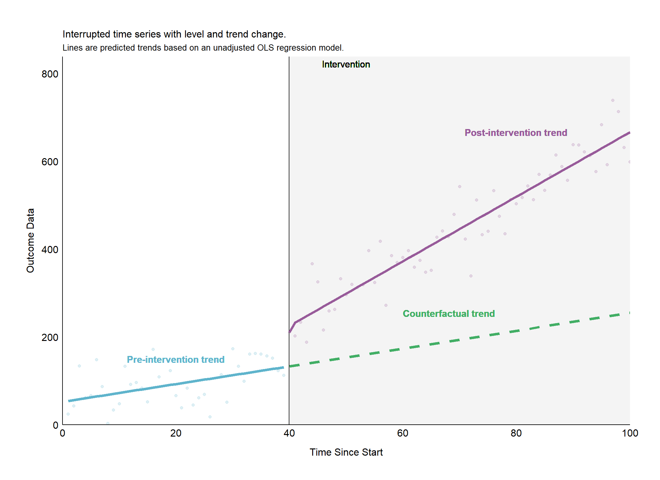
6.4 Interrupted Time Sries with Level and Trend Change
Reveal the Secret Within
library(ggplot2)library(tidyverse)library(lubridate) library(tidymodels) # --- Parameters ----outcome_baseline <-50pre_intervention_slope <-2level_shift <-100trend_change <-5interv_point <-40n_timepoints <-100# --- Simulation ----set.seed(123) base_data <-tibble(time =1:n_timepoints,outcome = outcome_baseline + pre_intervention_slope * time +rnorm(n_timepoints, 0, 50))# --- Apply Intervention Effects ----df_its <- base_data %>%mutate(outcome =ifelse(time >= interv_point, outcome + level_shift + trend_change * (time - interv_point), outcome) ) %>% dplyr::mutate(immediate =ifelse(time == interv_point,1,0),step =ifelse(time >= interv_point,1,0),ramp =ifelse(time > interv_point,time -1,0), )# --- Build Counter Factual Data and Predictions ----counter_factual_data <-tibble(time = interv_point:n_timepoints,immediate =0,step =0,ramp =0 )# --- Build OLS Model ----its_ols_model <- stats::lm(outcome ~ time + immediate + step + ramp , data = df_its)# --- Predict Counter Factual Trend ----counterfactual_trend <-predict(its_ols_model, counter_factual_data)# --- Prepare Plotting Lines ----pre_intervention_line <-tibble(time =1:(interv_point-1),outcome = its_ols_model$fitted.values[1:(interv_point-1)])post_intervention_line <-tibble(time = interv_point:n_timepoints,outcome = its_ols_model$fitted.values[interv_point:n_timepoints])counterfactual_line <-tibble(time = counter_factual_data$time,outcome = counterfactual_trend ) %>%slice(c(1, n()))# --- Build the Plot ----ggplot(df_its, aes(x = time, y = outcome)) +# Intervention Markergeom_vline(xintercept = interv_point, size =1, color ="grey10") +geom_rect( aes(xmin = interv_point, xmax = n_timepoints, ymin =-Inf, ymax =+Inf),fill ='grey95', alpha =0.2) +geom_text(aes(x = interv_point +10, y =+Inf, label ="Intervention",vjust =1.5, hjust =0.5),size =4,color ="black") +# Pre and Post Intervention Pointsgeom_point(data =filter(df_its, time < interv_point), color ="#5fb4cc", alpha =0.2) +geom_point(data =filter(df_its, time >= interv_point), color ="#985b9a", alpha =0.2) +# Lines (combined pre, post, and counterfactual for conciseness)geom_line(data = pre_intervention_line, color ="#5fb4cc", linetype ="solid",linewidth =1.5) +geom_line(data = post_intervention_line, color ="#985b9a",linetype ="solid",linewidth =1.5) +geom_line(data = counterfactual_line, color ="#42ae65", linetype ="dashed", linewidth =1.5) +# Trend Labels (adjusted positions for visual clarity)geom_text(aes(x = interv_point /2, y = outcome_baseline *3, label ="Pre-intervention trend"), color ="#5fb4cc", size =4, fontface ="bold") +geom_text(aes(x = n_timepoints *0.8, y =tail(post_intervention_line$outcome, 1), label ="Post-intervention trend"), color ="#985b9a", size =4, fontface ="bold") +geom_text(aes(x = n_timepoints *0.6, y =tail(counterfactual_line$outcome, 1),label ="Counterfactual trend"), color ="#42ae65", size =4, fontface ="bold", hjust =0) +# Theme customizationtheme_classic() +theme(# White background areaspanel.background =element_rect(fill ="white"),plot.background =element_rect(fill ="white"),plot.margin =unit(c(0.5, 0.5, 0.5, 0.5), "inches"),# Plot marginsplot.title =element_text(size =12,color ="black"),plot.subtitle =element_text(size =10,color ="black"),axis.title.y =element_text(size =12,color ="black", vjust =3),axis.title.x =element_text(size =12,color ="black", vjust =-3),axis.text =element_text(color ="black",size =12),# Remove axis ticksaxis.ticks =element_blank(),legend.position ="none" ) +ggtitle("Interrupted time series with level and trend change.", subtitle ="Lines are predicted trends based on an unadjusted OLS regression model.") +ylab("Outcome Data") +xlab("Time Since Start") +scale_y_continuous(expand =c(0, 0),breaks = scales::pretty_breaks(), limits =c(0,max(df_its$outcome)+100)) +scale_x_continuous(expand =c(0, 0),breaks = scales::pretty_breaks(), limits =c(0,n_timepoints))
Source Code
# Statistical Methods## Measuring EffectsIn order to measure the effects of an intervention, the immediate, step, and ramp effects are measured using statistical linear models. Using linear models to measure the effects in an interrupted time-series are useful for a few reasons.- **Interpretability:** The coefficients (β) have straightforward interpretations like baseline level, trend, and the magnitudes of different intervention effects.- **Underlying Trend:** Often, pre-intervention time series exhibit a roughly linear trend, making the linear model suitable.- **Flexibility:** Even with some non-linearity, the segmented structure of the model (pieces before and after the interruption) can still give a good approximation of change.## Linear EquationThe following equation is a common way to represent interrupted time series analysis in a statistical model.$$ \text{Yt} \sim \text{β0} + (\text{β1} * \text{T}) + (\text{β2} * \text{D}) + (\text{β3} * \text{P}) + \text{ϵ} $$- Each terms are explained below: - **Y_t:** The outcome you're measuring at time 't'. - **T:** Time, progressing incrementally throughout your study period. - **D:** A dummy variable, '0' before the intervention, '1' after, representing the intervention itself. - **P:** Time since the intervention, starting at 0 before the intervention. - **β_0:** The baseline trend of your outcome before the intervention and time. - **β_1:** The 'pre-intervention slope' of the outcome before the intervention. - **β_2:** The immediate change in the outcome level right at the point of intervention. - **β_3:** The difference in the trend (slope) between the pre-intervention and post-intervention periods (e.g., the difference in the slope after the intervention compared to the expected slope had the intervention not happened). - **ϵ:** Random error unaccounted for by the model.## Statistical ModelsThe choice of method can affect the level and slope change point estimates, their standard errors, width of confidence intervals, and p-values. Some possible choices include ordinary least squares (OLS), Newey-West (NW), Prais-Winsten (PW), restricted maximum likelihood (REML), and autoregressive integrated moving average (ARIMA) models.### Ordinary Least Squares (OLS)The classic linear regression model. It finds the line that best fits the data by minimizing the squared differences between observed values and predicted values. While usable for some ITS analysis, OLS is often problematic because time series data frequently violates the assumption of independent errors. Autocorrelation, if present, leads to underestimated standard errors and potentially misleading conclusions. OLS for ITS assumes residuals are independent (no autocorrelation) with constant variance.### Newey-West (NW)Also a linear regression method, but specifically designed to address autocorrelation. It adjusts the standard errors of the model coefficients to be robust to autocorrelation (and some heteroskedasticity). This gives more accurate assessments of statistical significance. A better choice than basic OLS when you suspect autocorrelation. However, it relies on the correct choice of lag structures.### Prais-Winsten (PW)Another way to handle autocorrelation. PW estimates a transformation of the model to remove autocorrelation (typically AR(1)) using a generalized least squares approach. Similar in spirit to NW, PW tends to be more efficient if the autocorrelation structure is correctly specified.### Restricted Maximum Likelihood (REML)REML targets estimating variance components rather than the regression coefficients themselves (like OLS). It produces less biased estimates of variance components than typical maximum likelihood approaches, especially in smaller samples. Relevant for ITS when you're using mixed-effects models with random intercepts/slopes to account for variability across different units or subgroups. REML helps get better estimates of these "group-level" effects.### Autoregressive Integrated Moving Average (ARIMA)ARIMA is useful for ITS if a trend needs to be modeled before and after the intervention, including forecasting potential continuing effects beyond the data (e.g., counter factual trend). Unlike the above methods, ARIMA explicitly models the dynamics of the time series itself. Specifically, ARIMA models accounts for the influence of past values on the current values with an autogressive component, handles differencing for non-stationary series, and incorporates lagged errors with a moving average. However, careful model selection is crucial. In this tutorial, we will use the `auto.arima()` function from the `forecast` package to choose an ARIMA model for us.## Interrupted Time Sries with Level and Trend Change```{r ITS-example-1,message = FALSE, warning=FALSE,error=FALSE,fig.dim = c(11, 8)}library(ggplot2)library(tidyverse)library(lubridate) library(tidymodels) # --- Parameters ----outcome_baseline <- 50 pre_intervention_slope <- 2 level_shift <- 100 trend_change <- 5 interv_point <- 40 n_timepoints <- 100 # --- Simulation ----set.seed(123) base_data <- tibble( time = 1:n_timepoints, outcome = outcome_baseline + pre_intervention_slope * time + rnorm(n_timepoints, 0, 50))# --- Apply Intervention Effects ----df_its <- base_data %>% mutate( outcome = ifelse(time >= interv_point, outcome + level_shift + trend_change * (time - interv_point), outcome) ) %>% dplyr::mutate( immediate = ifelse(time == interv_point,1,0), step = ifelse(time >= interv_point,1,0), ramp = ifelse(time > interv_point,time - 1,0), )# --- Build Counter Factual Data and Predictions ----counter_factual_data <- tibble( time = interv_point:n_timepoints, immediate = 0, step = 0, ramp = 0 )# --- Build OLS Model ----its_ols_model <- stats::lm(outcome ~ time + immediate + step + ramp , data = df_its)# --- Predict Counter Factual Trend ----counterfactual_trend <- predict(its_ols_model, counter_factual_data)# --- Prepare Plotting Lines ----pre_intervention_line <- tibble( time = 1:(interv_point-1), outcome = its_ols_model$fitted.values[1:(interv_point-1)])post_intervention_line <- tibble( time = interv_point:n_timepoints, outcome = its_ols_model$fitted.values[interv_point:n_timepoints])counterfactual_line <- tibble( time = counter_factual_data$time, outcome = counterfactual_trend ) %>% slice(c(1, n()))# --- Build the Plot ----ggplot(df_its, aes(x = time, y = outcome)) + # Intervention Marker geom_vline(xintercept = interv_point, size = 1, color = "grey10") + geom_rect( aes(xmin = interv_point, xmax = n_timepoints, ymin = -Inf, ymax = +Inf), fill = 'grey95', alpha = 0.2) + geom_text(aes(x = interv_point + 10, y =+Inf, label = "Intervention",vjust = 1.5, hjust = 0.5), size = 4,color = "black") + # Pre and Post Intervention Points geom_point(data = filter(df_its, time < interv_point), color = "#5fb4cc", alpha = 0.2) + geom_point(data = filter(df_its, time >= interv_point), color = "#985b9a", alpha = 0.2) + # Lines (combined pre, post, and counterfactual for conciseness) geom_line(data = pre_intervention_line, color = "#5fb4cc", linetype = "solid",linewidth = 1.5) + geom_line(data = post_intervention_line, color = "#985b9a",linetype = "solid",linewidth = 1.5) + geom_line(data = counterfactual_line, color = "#42ae65", linetype = "dashed", linewidth = 1.5) + # Trend Labels (adjusted positions for visual clarity) geom_text(aes(x = interv_point / 2, y = outcome_baseline * 3, label = "Pre-intervention trend"), color = "#5fb4cc", size =4, fontface = "bold") + geom_text(aes(x = n_timepoints * 0.8, y = tail(post_intervention_line$outcome, 1), label = "Post-intervention trend"), color = "#985b9a", size = 4, fontface = "bold") + geom_text(aes(x = n_timepoints * 0.6, y = tail(counterfactual_line$outcome, 1), label = "Counterfactual trend"), color = "#42ae65", size = 4, fontface = "bold", hjust = 0) + # Theme customization theme_classic() + theme( # White background areas panel.background = element_rect(fill = "white"), plot.background = element_rect(fill = "white"), plot.margin = unit(c(0.5, 0.5, 0.5, 0.5), "inches"), # Plot margins plot.title = element_text(size = 12,color = "black"), plot.subtitle = element_text(size = 10,color = "black"), axis.title.y = element_text(size = 12,color = "black", vjust = 3), axis.title.x = element_text(size = 12,color = "black", vjust = -3), axis.text = element_text(color = "black",size = 12), # Remove axis ticks axis.ticks = element_blank(), legend.position = "none" ) + ggtitle("Interrupted time series with level and trend change.", subtitle = "Lines are predicted trends based on an unadjusted OLS regression model.") + ylab("Outcome Data") + xlab("Time Since Start") + scale_y_continuous(expand = c(0, 0),breaks = scales::pretty_breaks(), limits = c(0,max(df_its$outcome)+100)) + scale_x_continuous(expand = c(0, 0),breaks = scales::pretty_breaks(), limits = c(0,n_timepoints)) ```